-->
Japanese
TOMIO KUROKAWA's WEB TOP PAGE.
Top
Current Recent Research Interests.
1. Graph Theory 2. Application of Graph Theory to Image Processing
3. Maze Construction Using Graph Theory & Image Processing 4. Genetic Algorithm Application to Image Processing & Graph Theory 5. Algorithm study over the above
Follwing are the Results of the Recent Research:
1 | ![]() |
The left picture is the checkered patterns generated using a computer program. Just given line drawn figures with Eulerian graph features, it produces various checkered patterns and their variations. Details of the algorithm are shown and a large number of experimental results are illustrated. Generation of checkered patterns |
2 | ![]() |
This is a Quiz maze to make a short sentence of English. "SOLVE MAZE" is the answer for this maze. Complex Picture Maze |
3 | ![]() |
Maze by One Stroke Drawing: The solution path is constructed along the drawn curve. However complex, it can be a maze if it is closed. Maze by One Stroke Drawing |
4 | ![]() |
Picture Maze with Contours: The maze solution paht is constructed by connecting the contours of pictures such as letters. Very complex maze can be generated. Picture Maze along Contours |
5 | ![]() |
Picture Maze by Hamiltonian PathFThe solution is a Hamiltonian path. It is constructed by successive insertions of a small unit path thought the foreground part of pictures such as letters or symbols. The construction is made very fast by the direct insertion of the unit path. The diagram on the left is without the dead-end branches. Picture Maze by Hamiltonian Path |
6 | ![]() |
Picture Maze by near Hamiltonian Path: The solution is not a complete Hamiltonian path. The path is constructed by successive insertions of a small unit path. But the unit is smaller than that used for Hamiltonian path construction. The construction is very fast for the same reason above. Picture Maze by near Hamiltonian Path |
Checkered Patterns 1 | Checkered Patterns 2 | Checkered Patterns 3 | |
![]() |
![]() |
![]() |
|
Checkered Patterns 4 | Checkered Patterns 5 | Checkered Patterns 6 | |
![]() |
![]() |
![]() |
|
Checkered Patterns 7 | Checkered Patterns 8 | Checkered Patterns 9 | |
![]() |
![]() |
![]() |
|
All of the above-checkered patterns were generated in the following manner. 1. Draw a figure with closed path curves (overlapped closed curves). 2. Extract the contours of the above. 3. Bipartite the contours into two sets. 4. Paint the contour surrounded regions of each set with a color --- producing the checkered patterns. Refer to the following for details: Tomio Kurokawa, "Generation of Checkered Patterns and Their Variations by Making Use of Eulerian Graph Features," British Journal of Mathematics & Computer Science, Vol.20, Issue.3, pp.1-29, 2017.1, SCIENCEDOMAIN international, ISSN: 2231-0851, http://sciencedomain.org/issue/2067 Paper download - DOI:https://doi.org/10.9734/BJMCS/2017/30783 |
Figure 1 | Figure 2 | Figure 3 | Figure 4 |
![]() |
![]() |
![]() |
![]() |
Original Picture: Two rectangles are drawn with thin lines crossed each other. | Contours are extracted from Figure 1. These contour lines are on the lines of the original figure. Each contour surrounds the region surrounded by the original figure lines. They (or surrounded regions) are numbered. | The regions are considered as graph vertices and an edge is drawn between the two vertices if two regions are adjacent. This graph is called region adjacency graph, RAG, which is drawn yellow. This step of drawing RAG is not necessary for checkered pattern generation. The required action is just to separate the contours into two sets (X and Y), bi-partitioning. | The contours in partition X are shown. Contours in X and Y are shown in Figure 3. They are overlapped very where. So the contours in X only looks the same as Figure 3. |
Figure 5 | Figure 6 | Figure 7 | |
![]() |
![]() |
![]() |
|
The contours in partition Y are shown. As the same reason, contours in Y only look like Figure 3, too. | After all the adjacencies are examined, the bipartite graph can be drawn as in this figure. But this drawing is not required for the checkered pattern generation. | The checkered patterns are completed. The regions surrounded by the contours in X are colored yellow; those in Y and on boundaries by yellow. | Other checkered patterns can be generated by the above process. |
Refer to the following for details: Tomio Kurokawa, "Generation of Checkered Patterns and Their Variations by Making Use of Eulerian Graph Features," British Journal of Mathematics & Computer Science, Vol.20, Issue.3, pp.1-29, 2017.1, SCIENCEDOMAIN international, ISSN: 2231-0851, http://sciencedomain.org/issue/2067 Paper download-DOI:https://doi.org/10.9734/BJMCS/2017/30783 |
1 | ![]() |
To construct the maze here, we first organize a path which visits all the image dots, each only once with no intersection between connecting lines and dots; then construct a near-Hamiltonian path within each of image dots, which completes the solution path of the maze. Adding the dead-end branches and thinning the walls of the maze complete the maze that is to be presented to players. The maze on the left shows the maze as well as the solution path painted as red. | |
2 | ![]() |
The maze on the left is the one where dots are replaced with English letters, an English word quiz. The answer is "SOLVE MAZE". | |
Refer to the paper below for details. Tomio Kurokawa, "Construction of Picture Maze along Set of Image Dot Vertices," British Journal of Mathematics & Computer Science, Vol.17, Issue.1, pp.1-14, 2016.5, SCIENCEDOMAIN international, UK, ISSN: 2231-0851, http://sciencedomain.org/issue/1786 Paper Down Load-DOI:https://doi.org/10.9734/BJMCS/2016/26350 |
1 |
![]() |
![]() |
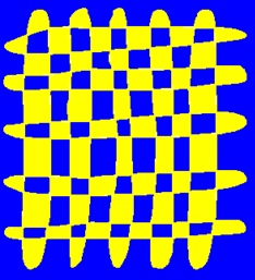
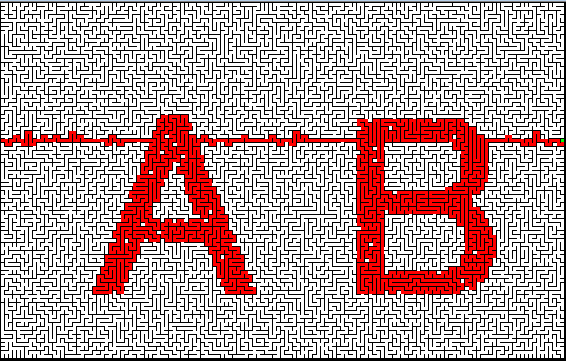
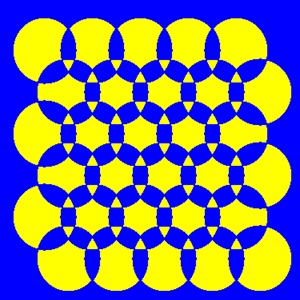
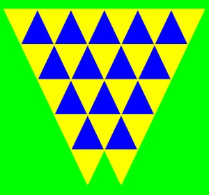
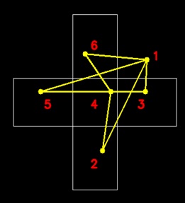
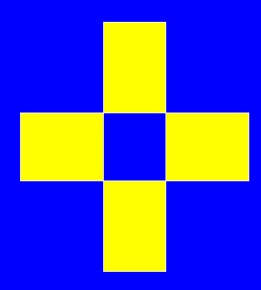
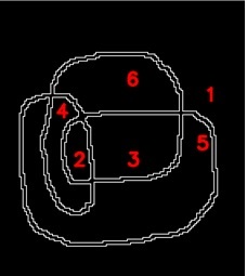
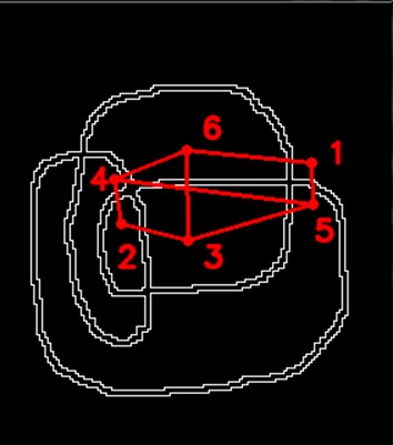
The left side of these two left pictures is the one stroke closed curve with line width of 3 pixels, rather wide. .
The right picture is the contours of the curve extracted; all the contours are cycles and numbered, 1 to 6.
Every part of the original curve is covered by two cycle lines. If the curve of the original curve is narrow, one pixel or less, the double contour cycles are expected to overlap. If we consider the intersection of the curve as a vertex and the curve between two vertices as an edge of a graph, the closed curve can be considered as a graph with every vertex of even degree. Therefore, the graph is Eulerian. The overlapped cycles occupy the same vertices and the edges and organize two Eulerian circuits. However, the path routes of the two are different. Considering the region surrounded by the original curve as a vertex and the adjacency between the two vertices as an edge, we have a graph, which is known to be a bipartite graph. By the same way, consider the region surrounded by a cycle as a vertex and the adjacency between two cycles as an edge, we have a graph. We name the graph as the region cycle graph. By analogy, this graph should be a bipartite graph. So it is possible to separate the cycles into two sets, partition X and partition Y. This means that every point on the original curve has the corresponding point on each of the cycle sets. This enables the construction of the two Eulerian circuits. |
2 |
![]() |
![]() |
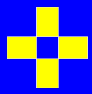
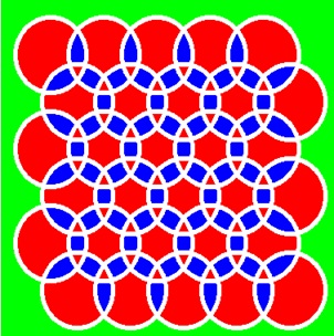
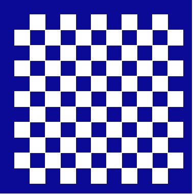
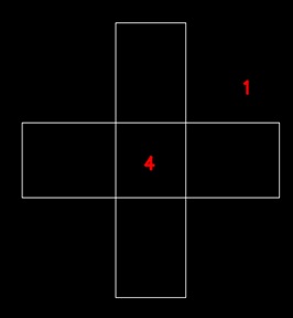
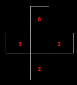
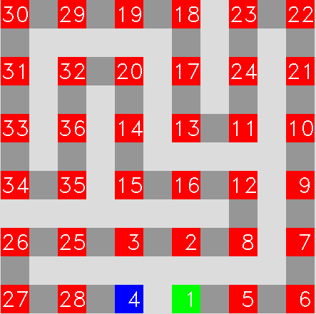
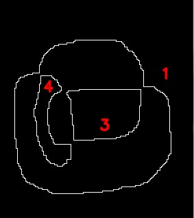
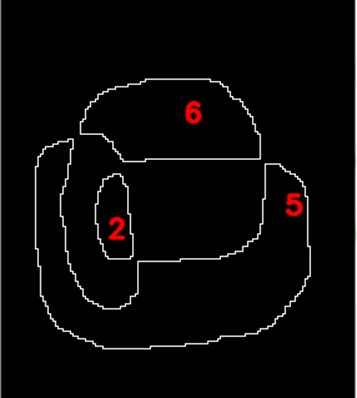
The figures on the left are the two partitions of cycle sets |
3 |
![]() |
![]() |
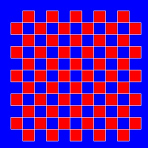
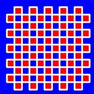
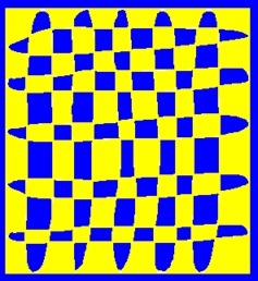
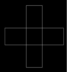
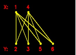
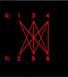
The left of the left is the bipartite graph of the cycles extracted. The right of the left is the region cycle graph, a bipartite graph, previously explained. |
4 |
![]() |
![]() |
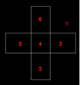
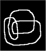
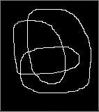
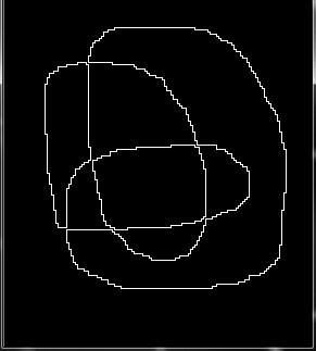
The left of the left is the one stroke closed drawing with line width of one pixel. The right of the above is the contours extracted from the picture. Every part of the curve is covered by the double contour cycles like the previous case with 3 pixel line width. However, the contours look like single lines. This is because those contour lines overlap at most of the original curve. |
5 |
![]() |
![]() |
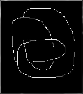
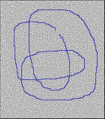
The same procedure of the bi-partitioning was applied the contour cycles of one pixel width. The results are the cycles shown on the left two figures. Both look alike. However, they are different cycle sets. One is composed of the five cycles and the other three cycles. This is more persuasive to say that the contours of a one stroke closed curve constitute two Eulerian circuits. |
6 |
![]() |
![]() |
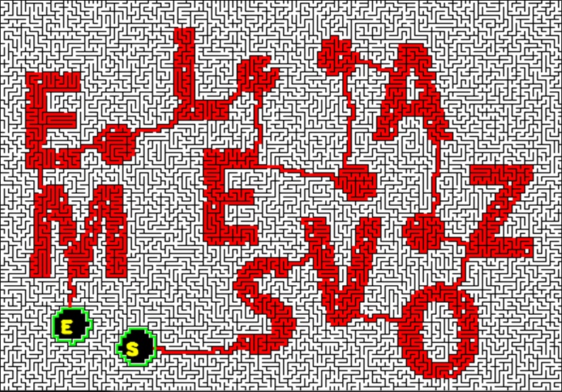
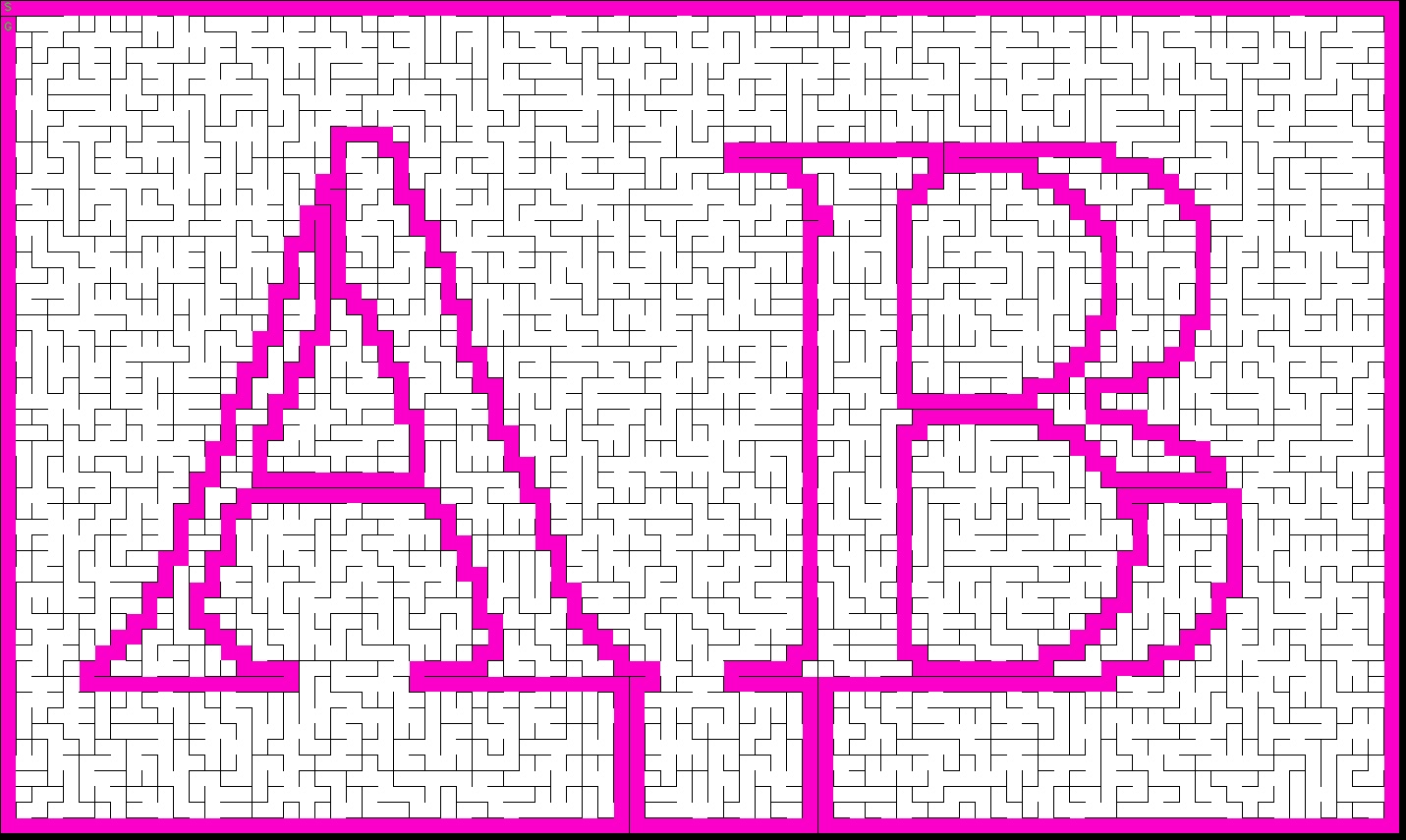
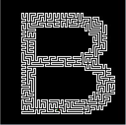
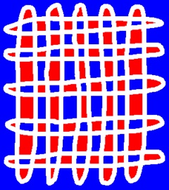
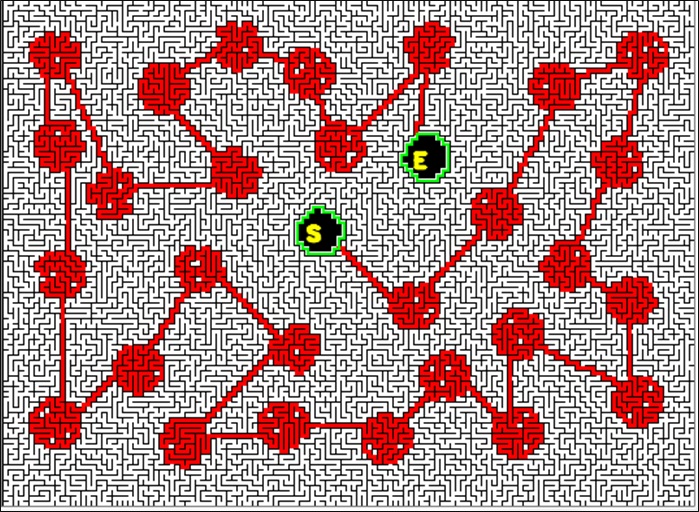
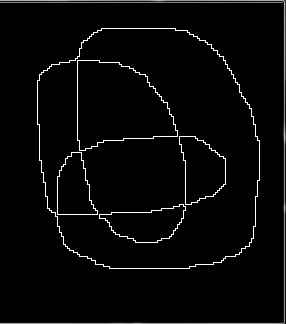
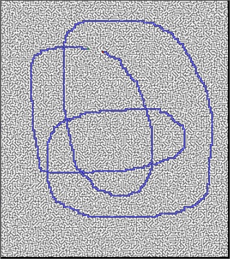
Each of the previous partitions of X and Y was merged into one single cycles. A part of the route was cut to designate the ends as the start and the goal of the maze path. Adding some random dead end branches and thinning the walls complete the mazes, which are shown on the left. Both, X and Y, look alike but have different path routes. |
7 |
Refer to the paper below for the details. Tomio Kurokawa, "Maze Construction by Using Characteristics of Eulerian Graphs," British Journal of Mathematics & Computer Science, Vol.9, Issue.6, pp.453-472, 2015.6, SCIENCEDOMAIN international, UK, ISSN: 2231-0851, http://sciencedomain.org/issue/1147 Paper Down Load-DOI:https://doi.org/10.9734/BJMCS/2015/18125 |
1 | ![]() |
Picture maze is the kind of maze on which some picture appears when the solution is given.
Considering the letters "AB" as a picture,
the left figure shows the solution path for the maze under which "AB" was varied. The maze is constructed as follows: 1) Contours are extracted for the picture "AB"; the each contours are cycles. 2) The outer frame path is introduced; start and goal are specified at the upper left conner. 3) Those contours are successively merged so that a single cycle is organized. 4) Random dead end branches are added to the solution path: 5) Procedure finishes. | |
2 | ![]() |
It is possible to generate a picture maze from a very complicated binary picture such as the left. | |
For more detail, refer to the document below: Tomio Kurokawa, "Picture Maze Generation by Repeated Contour Connection and Graph Structure of Maze," Computer Science and Engineering, Vol.3, No.3, pp.76-83, 2013.12, Scientific & Academic Publishing, USA , ISSN:2163-1484 http://article.sapub.org/10.5923.j.computer.20130303.04.html Paper Down Load |
1 | ![]() |
The left hand figure shows the solution path for the maze under which the letter "B" is buried.
The path is so organized that it goes through each cell once on all cells of the picture of "B."
This kind of path is called Hamiltonian path.
The figure illustrates only the solution path not including the random branch paths.
To complete the maze, however,
those random branches have to be incorporated and walls must be thinned so that the player can handle it easier.
Since the path goes through all part of the picture,
the picture should appear when the player solves it. To construct the maze solution path, the following steps are necessary: 1) The original picture is expanded by 2*2 so that Hamiltonian path can be constructed on the picture. 2) the initial block path is set with start and goal; 3) then a path segment is repeatedly inserted into the path being constructed until no space is left on the picture "B". |
|
2 | ![]() |
The left hand figure illustrates the Hamiltonian path within a square region. The path construction starts with the initial block path which only goes through "1", "2", "3" and "4" in this order. "1" is the start and "4" is the goal. The first insertion of the path segment is done between the "1" and "2." Next is between "7 "and "8." Accordingly, the insertion is repeated until no space is left in the region. The path going through all the vertices in the region completes. | |
3 | ![]() |
The left hand two figures are for the detailed explanation for the path construction of the figure 3. The method of the path generation makes a Hamiltonian path. A brief simple proof by mathematical industion is given below: 1) The initial path can be constructed as long as the space exists. 2) Suppose a Hamiltonian path is completed within the region of n blocks. 3) As long as a space exists, it must be adjacent to the path of the n block because the region is connected. Therefore n plus 1st block path can be always inserted to the path. This complete the proof. |
|
4 | ![]() |
||
For more detail, refer to the document below: Tomio Kurokawa, "Picture Maze Generation by Successive Insertion of Path Segment," British Journal of Mathematics & Computer Science, Vol.4, Issue.24, pp.3444-3463, 2014.12, SCIECEDOMAIN international, UK, ISSN: 2231-0851 http://www.sciencedomain.org/issue.php?iid=699&id=6 Paper Download-DOI:https://doi.org/10.9734/BJMCS/2014/12048 |
1 | ![]() |
The left hand figure illustrates the maze solution path (red) for the picture "AB."
This path is not a Hamiltonian path.
The path is constructed without the initial picture expansion of 2*2.
So there is no guarantee that a Hamiltonian path can be generated.
The construction procedure is as follows: 1) The initial path is constructed crossing "A" and "B" all the way through from the right to the left. 2) The path insertion is made repeatedly within the picture regions of "A" and "B." But for this case, the block path to be insterted is only includes two vertices instead of four. 3) When the path occupies almost all spaces in the region of "A" and "B," the path extension is stopped. 4) A small number of path extensions are applied to the path segment not on "A" and "B." This completes the path. 5) The path is shown in red in the figure. |
|
For more detail, refer to the document below: Tomio Kurokawa, "Picture Maze Generation by Successive Insertion of Path Segment," British Journal of Mathematics & Computer Science, Vol.4, Issue.24, pp.3444-3463, 2014.12, SCIECEDOMAIN international, UK, ISSN: 2231-0851 http://www.sciencedomain.org/issue.php?iid=699&id=6 Paper Download-DOI:https://doi.org/10.9734/BJMCS/2014/12048 |